×
What's this?
Accounts have been assigned only to users involved in the annotation process. If you believe you need an account, please contact Nicholas Heller at helle246@umn.edu.
What's this?
Accounts have been assigned only to users involved in the annotation process. If you believe you need an account, please contact Nicholas Heller at helle246@umn.edu.
The 2021 Kidney and Kidney Tumor Segmentation challenge (abbreviated KiTS21) is a competition in which teams compete to develop the best system for automatic semantic segmentation of renal tumors and surrounding anatomy.
Kidney cancer is one of the most common malignancies in adults around the world, and its incidence is thought to be increasing [1]. Fortunately, most kidney tumors are discovered early while they’re still localized and operable. However, there are important questions concerning management of localized kidney tumors that remain unanswered [2], and metastatic renal cancer remains almost uniformly fatal [3].
Kidney tumors are notorious for their conspicuous appearance in computed tomography (CT) imaging, and this has enabled important work by radiologists and surgeons to study the relationship between tumor size, shape, and appearance and its prospects for treatment [4,5,6]. It’s laborious work, however, and it relies on assessments that are often subjective and imprecise.
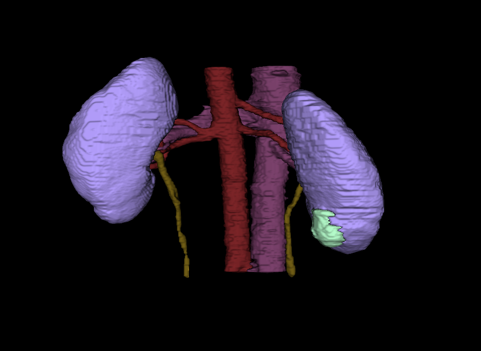
Automatic segmentation of renal tumors and surrounding anatomy (Fig. 1) is a promising tool for addressing these limitations: Segmentation-based assessments are objective and necessarily well-defined, and automation eliminates all effort save for the click of a button. Expanding on the 2019 Kidney Tumor Segmentation Challenge [7], KiTS21 aims to accelerate the development of reliable tools to address this need, while also serving as a high-quality benchmark for competing approaches to segmentation methods generally.
| Mar 1 - Jul 1 | Annotation, Release, and Refinement of Training Data |
| Aug 23 | Deadline for Intention to Submit & Required Paper (formerly Aug 9) |
| Aug 30 - Sep 17 | Submissions Accepted (formerly Aug 16 - Aug 30) |
| Sep 21 | Results Announced (formerly Sep 1) |
| Sep 27 | Satellite Event at MICCAI 2021 |
The KiTS21 cohort includes patients who underwent partial or radical nephrectomy for suspected renal malignancy between 2010 and 2020 at either an M Health Fairview or Cleveland Clinic medical center. A retrospective review of these cases was conducted to identify all patients who had undergone a contrast-enhanced preoperative CT scan that includes the entirety of all kidneys.
Each case's most recent corticomedullary preoperative scan was (or will be) independently segmented three times for each instance of the following semantic classes.
We are hard at work on collecting and annotating data for KiTS21. At this point it's difficult to predict the total number of patients that KiTS21 will include. We had originally aimed to segment 800 cases, but unfortunately the COVID19 global pandemic has delayed our progress. We plan to continue collecting and annotating training cases right up until the training set is "frozen" released on July 1, 2021. After this point, we will continue to collect and annotate cases for the test set until submissions begin in the middle of August. Training set annotation progress can be tracked using the Browse feature, described in detail in the section below. The training set will not be "frozen" until two weeks after release.
In an effort to be as transparent as possible, we've decided to perform our training set annotations in full view of the public. This is the primary reason for creating an independent website for KiTS21 on top of our grand-challenge.org entry, which will be used only to manage the submission process.
You may have noticed a link on the top-right of this page labeled "Browse". This will take you to a list of the KiTS21 training cases, where each case has indicators for its status in the annotation process (e.g., see Fig. 3). The meaning of each symbol is as follows:
When you click on an icon, you will be taken to an instance of the ULabel Annotation Tool where you can see the raw annotations made by our annotation team. Only logged-in members of the annotation team can submit their changes to the server, but you may make edits and save them locally. The annotation team's progress is synced with the KiTS21 GitHub repository about once per week.
It's important to note the distinction between what we call "annotations" and what we call "segmentations". We use "annotations" to refer to the raw vectorized interactions that the user generates during an annotation session. A "segmentation," on the other hand, refers to the rasterized output of a postprocessing script that uses "annotations" to define regions of interest.
We placed members of our annotation team into three categories:
Broadly, our annotation process is as follows.
Our postprocessing script uses thresholds and fairly simple heuristic-based geometric algorithms. Its source code is available on the KiTS21 GitHub repository under /kits21/annotation/postprocessing.py.
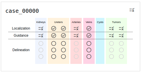
Fig. 3: An example of a case in progress as it's listed on the browse page. The icon on the top right indicates the status of region detection, and its current value signals that it needs review. Similar icons are used to show the status of each region individually. Ureters, Arteries, and Veins are now extraneous for KiTS21 and can be ignored.
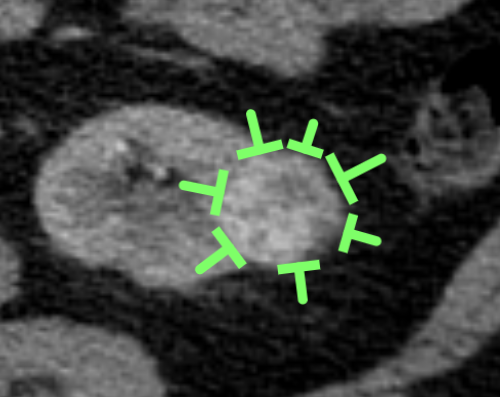
Fig. 4: "Guidance pins" that were placed by medical students to show intention to annotate a tumor for an eventual worker on mechanical turk.
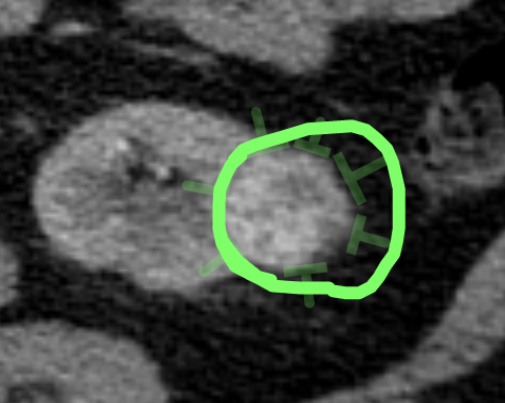
Fig. 5: Contour drawn by a crowdworker based on the guidance pins drawn by a medical student. The "excess" sinus fat included in the contour is removed automatically via a radiodensity threshold during postprocessing.
This section was changed substantially on July 16, 2021. Show prior version
Put simply, the model that produces the "best" segmentations of kidneys, tumors, and cysts for the patients in the test set will be declared the winner. Unfortunately "best" can be difficult to define [8].
Before metrics are discussed, we need to discuss the regions that they will be applied to. A common choice in multiclass segmentation is to simply compute the metric for each semantic class and take the average. For this challenge, we don't think this is the best approach. To illustrate why, consider a case in the test set where a single kidney holds both a tumor and a cyst. If a submission has a very high-quality kidney segmentation, but struggles to differentiate kidney voxels from those belonging to the masses, we believe this deserves a high score for the kidney region, but low scores for each mass. Similarly, suppose the masses were segmented nicely, but the system confuses the cyst with the tumor. We don't think it is ideal to penalize the submission twice here (one for the tumor region, once for the cyst region) when in fact it has done a very good job segmenting masses. To address this, we use what we call "Hierarchical Evaluation Classes" (HECs). In an HEC, classes that are considered subsets of another class are combined with that class for the purposes of computing a metric for the superset. For KiTS21, the following HECs will be used.
In 2019, we used a simple Sørensen-Dice ranking with "Kidney and Tumor", and "Tumor" HECs. The decision to use Dice alone was made to prioritize simplicity and ease of interpretation. We still believe that these things are important, but we also recognize that Dice scores have their limitations. One limitation was the outsized influence that small tumors had on the rankings. This was because segmentation errors are overwhelmingly on the borders of regions, and small regions have a higher ratio of border voxels to interior voxels, leading to lower values for volumetric overlap scores like Dice.
In order to address this, we had originally planned to use "Gauged Scores", which take into account the interobserver agreement on a case and scale the metric accordingly. However, after some internal experiments, we realized that this approach was ill-suited for this particular segmentation task. The primary reason was that our "interobserver agreement" was inflated due to the shared "guidance pins" that the annotators were using as references. This resulted in gauged scores that suggested extremely poor performance in relation to the humans, when in fact the predictions often looked (qualitatively) equally good if not better.
In addition, we had originally proposed to use the surface-distance-based metrics of RMSD and ASSD for each of our HECs and then aggregate their gauged values with those of the volumetric overlap scores via averaging. We have decided that this, too, is ill-suited for our problem because these penalize false positive/negative predictions by their distance rather than their existence. While this property is useful for organ segmentation, it is not desired for tumor segmentation where lesions can be spread throughout the affected organ and thus do not have an expected spatial location.
Given that, we have decided to use only two metrics this year:
These will be computed for every HEC of every case of the test set on a random sample of aggregated segmentations created using the logic implemented in /kits21/annotation/sample_segmentations.py.
The metrics will be averaged over each HEC, and then teams will be ranked based on both average metrics. The final leaderboard place will be determined by averaging the leaderboard places between the two rankings, sometimes called "rank-then-aggregate". In the case of any ties, average Sørensen-Dice value on the "Tumor" HEC will be used as a tiebreaker.
An implementation of these metrics and ranking procedure can be found at /kits21/evaluation/.
You are viewing an out-of-date version of this section. Show current version
Put simply, the model that produces the "best" segmentations of kidneys, tumors, and cysts for the patients in the test set will be declared the winner. Unfortunately "best" can be difficult to define [8].
Before metrics are discussed, we need to discuss the regions that they will be applied to. A common choice in multiclass segmentation is to simply compute the metric for each semantic class and take the average. For this challenge, we don't think this is the best approach. To illustrate why, consider a case in the test set where a single kidney holds both a tumor and a cyst. If a submission has a very high-quality kidney segmentation, but struggles to differentiate kidney voxels from those belonging to the masses, we believe this deserves a high score for the kidney region, but low scores for each mass. Similarly, suppose the masses were segmented nicely, but the system confuses the cyst with the tumor. We don't think it is ideal to penalize the submission twice here (one for the tumor region, once for the cyst region) when in fact it has done a very good job segmenting masses. To address this, we use what we call "Hierarchical Evaluation Classes" (HECs). In an HEC, classes that are considered subsets of another class are combined with that class for the purposes of computing a metric for the superset. For KiTS21, the following HECs will be used.
In 2019, we used a simple Sørensen-Dice ranking with "Kidney and Tumor", and "Tumor" HECs. The decision to use Dice alone was made to prioritize simplicity and ease of interpretation. We still believe that these things are important, but we also recognize that Dice scores have their limitations. One limitation was the outsized influence that small tumors had on the rankings. This was because segmentation errors are overwhelmingly on the borders of regions, and small regions have a higher ratio of border voxels to interior voxels, leading to lower values for volumetric overlap scores like Dice.
NOTE: After internal experiments, we have decided to revise our approach to evaluation. This section will be updated shortly with new information. The test set is being annotated using an identical workflow as that used for the training set, and so it too will have several segmentations per case. We've decided to take advantage of this in order to address some of the limitations of a single-reference Dice approach. Our planned approach is similar to that of Heimann et al. for liver segmentation in the 2007 MICCAI Challenge Workshop [9]. In particular, we will be computing gauged scores for each predicted region, which are adjusted according to the average error observed between human raters in that region.
Formally, let  be the error between the prediction and reference, where the subscripts represent:
 : The case number of the scan in the test set that these regions were pulled from.
 : The index of the hierarchical evaluation class that these regions are meant to represent.
 : The index of the set of raters who created the reference.
 : The metric used to compute error (1-6 corresponding to the table with six metrics below).
Similarly, let  represent the average error between rater and the remaining two raters. Submissions will be ranked according to a total score
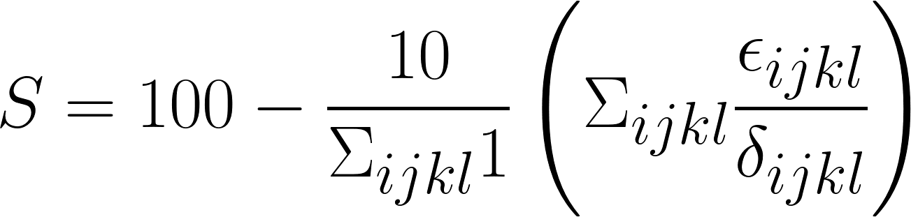
The intent of this transformation is to normalize scores so that predictions with roughly equal quality to that of our trainees will achieve a score of  . Note that negative scores are possible where error is at least 10 times as high as it is between trainees on average. The six metrics to be used (tentatively) for this computation are as follows:
| 1 - Dice |
A common measure of discrepancy in volumetric overlap. If we let  be the set of predicted voxels and be the set of predicted voxels and  be the set of reference voxels, be the set of reference voxels,

|
| 1 - IoU |
Sometimes referred to as 1 - Jaccard. Another measure of discrepancy in volumetric overlap, with a greater emphasis on cases with high disagreement.

|
| Symmetric Relative Volume Difference |
A measure of difference in total predicted volume, but slightly modified from traditional Relative Volume Difference.

|
| Absolute Volume Difference |
Another measure of difference in total predicted volume, but without normalizing for the size of the reference. Using our notation from above,

|
| Average Symmetric Surface Distance |
The average distance between each prediction boundary voxel to the nearest boundary voxel of the reference, and vice versa. Boundary voxels are defined as any voxel in a region that has a voxel outside of that region in its 18-neighborhood. Let  and and  represent the sets of boundary voxels on the prediction and reference sets respectively. represent the sets of boundary voxels on the prediction and reference sets respectively.
 where
where

|
| RMS Symmetric Surface Distance |
Similar to average symmetric surface distance, but with greater emphasis on boundary areas with large disagreement.

|
In the occasional cases where either a reference HEC or a predicted HEC is empty but not both, the metrics will be computed as follows:
 will be set to 1.
 will be set to 1.
 will be zero if the prediction is empty. If an erroneous prediction is made, the gauge error will be set to 1 divided by the proportion of instances for which the annotators made the same mistake on that region during step 1 of the annotation process (and the mistake was discovered during review).
 will be set to 1 times the volume, and the gauge error will be computed by setting
  to the average volume of regions in that class.
 will be set to 10cm (the max possible).
 will be set to 10cm (the max possible).
The above treatment of the volume-difference-based scores was derived such that human annotators would be expected to achieve a total score of roughly 90 on cases with empty references, since that is also the intention with nonempty cases. It's also somewhat intuitive since it consists of a flat penalty for the false positive/negative plus an additional term that increases with the size of the region that was missed or erroneously predicted. In cases where both the predicted and reference HEC are empty, all errors will be set to zero.
The code that will be used to compute these metrics on the test set will be available on the GitHub repository under /kits21/evaluation/ (in preparation).
This project is a collaboration between the University of Minnesota Robotics Institute (MnRI), the Helmholtz Imaging Platform (HIP) at the German Cancer Research Center (DKFZ), and the Cleveland Clinic's Urologic Cancer Program.
 Histosonics, Inc. has sponsored a $5000 prize for the team that places first on the official leaderboard.
 Intuitive Surgical has graciously provided funding which partially supported the annotation process for the KiTS21 data.
 This challenge was made possible by scholarships provided by Climb 4 Kidney Cancer (C4KC), an organization dedicated to advocacy for kidney cancer patients and the advancement of kidney cancer research.
 This work was also supported by the National Cancer Institute of the National Institutes of Health under Award Number R01CA225435.